Calibration

The problem

The market quotes prices $m_1, \dots, m_n$ of European options with strikes $K_i$ and maturities $T_i$: here 13 strikes on each of four maturities, out of the money (puts below the forward, calls above it), whose prices hold no intrinsic value. Their implied volatilities $v_i$ invert the formula of Black and Scholes $C_{bs}$: $C_{bs}(S_0, K_i, r, T_i, v_i, d) = m_i$. MarketData holds them as a matrix, one row per maturity.

A model with parameters $p$ gives the prices $C_i(p)$, computed with the pricer of FinancialMonteCarlo by any pricing method, one smile per maturity. Their implied volatilities $\sigma_i(p)$ are the model volatilities, and the calibration minimises the volatility errors

\[e_i(p) = \sigma_i(p) - v_i, \qquad L(p, v) = \frac{1}{2} \sum_{i=1}^n e_i(p)^2 .\]

Volatilities rather than prices put the errors of all the strikes on one scale: the price of a far out of the money option is a small number, and an error on it of the size of the error at the money would be a large error in volatility. vol_errors returns $e(p)$, and FinancialCalibrator.loss returns $L$.

Which quotes enter $L$ is decided once, on the quotes: only out of the money options (an in the money option is mostly intrinsic value, and its implied volatility is ill-conditioned), and only those whose vega at the quoted volatility is at least min_vega times the spot (1e-3 by default): a price far below the accuracy of the pricing method gives an implied volatility that moves erratically with the parameters, and a loss that is not smooth.

The model is Heston's, with the variance $V$ of the log-price mean-reverting at the speed $\kappa$ to the level $\theta$,

\[\frac{dS_t}{S_t} = (r - d)\,dt + \sqrt{V_t}\,dW_t, \qquad dV_t = \kappa (\theta - V_t)\,dt + \sigma \sqrt{V_t}\,dZ_t, \qquad d\langle W, Z\rangle_t = \rho\,dt, \qquad V_0 = \sigma_0^2,\]

HestonProcess(σ, σ₀, λ, κ, ρ, θ, underlying), with no market price of volatility risk ($\lambda = 0$). The quotes are generated by the model itself, with $p = (0.5, 0.2, 1.5, -0.7, 0.04)$, and their prices are moved by up to 1%, which no Heston model fits exactly.

using FinancialCalibrator, FinancialMonteCarlo, FinancialFFT, FinancialToolbox, ForwardDiff, LinearAlgebra, Dates

S0, r, d = 100.0, 0.02, 0.01
zero_rate = ZeroRate(r)
underlying = Underlying(S0, d)
maturities = [0.25, 0.5, 1.0, 2.0]
strikes = collect(70.0:5.0:130.0)
forward(T) = S0 * exp((r - d) * T)

# the quotes: out of the money prices of the model, moved by up to 1%, and their implied volatilities
method = CosMethod(2^9)
heston_market = HestonProcess(0.5, 0.2, 0.0, 1.5, -0.7, 0.04, underlying)
function quoted_vols(T, row)
    calls = strikes .>= forward(T)
    prices = pricer(heston_market, zero_rate, method, FinancialMonteCarlo.EuropeanOptionSmile(T, strikes, calls))
    prices = prices .* (1 .+ 0.01 .* sin.((row - 1) * length(strikes) .+ (1:length(strikes))))
    return blsimpv.(S0, strikes, r, T, prices, d, calls)
end
vols = reduce(vcat, [permutedims(quoted_vols(T, i)) for (i, T) in enumerate(maturities)])
mkt = MarketData(maturities, [Date(2026) + Day(round(Int, 365 * T)) for T in maturities], fill(r, length(maturities)), strikes, vols)

The variables of the search

The parameters are constrained: $\sigma$, $\sigma_0$, $\kappa$ and $\theta$ are positive, and $|\rho| < 1$; and $\lambda$ is not determined by the quotes at all, since only $\kappa + \lambda$ enters the prices. A Parametrization searches over unconstrained variables $x$, with $p = (e^{x_1}, e^{x_2}, 0, e^{x_3}, \tanh x_4, e^{x_5})$, so that every step gives a valid model, and $\lambda$ stays at zero. This is also default_parametrization of a Heston model, which the calibration uses when no parametrization is given; it is spelled out here to show how one is written:

variables = Parametrization(x -> [exp(x[1]), exp(x[2]), zero(x[1]), exp(x[3]), tanh(x[4]), exp(x[5])],
                            p -> [log(p[1]), log(p[2]), log(p[4]), atanh(p[5]), log(p[6])])
start = HestonProcess(0.3, 0.25, 0.0, 1.0, -0.3, 0.06, underlying)

The search starts from the parameters of start.

Derivatives of the model volatilities

The model volatility $\sigma_i(p)$ solves $C_{bs}(S_0, K_i, r, T_i, \sigma_i, d) = C_i(p)$. By the implicit function theorem its derivatives are those of the price, divided by the vega $\nu_i = \partial_\sigma C_{bs}$ at $\sigma_i$:

\[\frac{\partial \sigma_i}{\partial p_j} = \frac{1}{\nu_i} \frac{\partial C_i}{\partial p_j},\]

and this is how the rules of blsimpv (FinancialToolbox) differentiate it, without going through the iterations of its solver. The Jacobian $J = \partial_x e$ of the errors is then one evaluation of the pricer in dual numbers, through the characteristic exponent, the pricing method and the implied volatility.

Levenberg–Marquardt

calibrate minimises $L$ in two stages. An Optim optimizer (NelderMead() by default; any other, with its options, as the fourth and fifth arguments) finds the basin; Levenberg–Marquardt then brings the solution to where the gradient of $L$ vanishes, which an optimizer stopped by its own tolerances does not reach, and which the sensitivities below need. The default options stop the optimizer early (g_tol = 1e-6, against Optim's 1e-8), since the polish converges from there in a few steps: on DAX the same optimum for every model tried, in half the time for Kou and Merton. Where the parameters cannot be priced, $L = \infty$, which the optimizer ranks as the worst point. Gauss–Newton linearises the errors around the current point, $e(x + \delta) \approx e(x) + J \delta$, and takes the least squares solution of $J \delta = -e$. Levenberg and Marquardt add a damping $\mu > 0$:

\[\left(J^\top J + \mu D\right) \delta = -J^\top e, \qquad D = \operatorname{diag}\left(J^\top J\right).\]

For $\mu \to 0$ the step is the Gauss–Newton one; for a large $\mu$ it is a short step along the gradient $-J^\top e$ of the loss, scaled by $D$ (Marquardt's choice, which makes the step independent of the units of the parameters). $\mu$ is divided after a step that decreases the loss, which is accepted, and multiplied after one that does not, or whose parameters are invalid (the pricing throws), which is rejected.

res = calibrate(start, method, mkt; parametrization = variables, min_vega = 0)
p = res.OptimalParam
(market = [0.5, 0.2, 0.0, 1.5, -0.7, 0.04], calibrated = p, rms_error = sqrt(2 * res.OptimalValue / length(vols)))

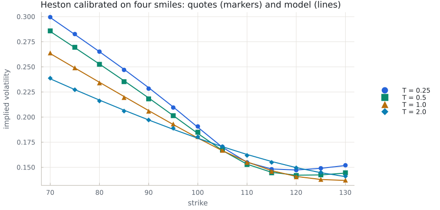
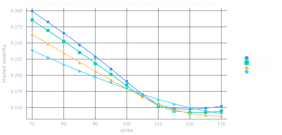
(market = [0.5, 0.2, 0.0, 1.5, -0.7, 0.04], calibrated = [0.49747564363765245, 0.2003220236312285, 0.0, 1.4997213211330764, -0.7015077269964037, 0.03991901103577728], rms_error = 0.0006294941839232573)

min_vega = 0 keeps every quote, as the FinancialFFT page does. The root mean square error is about 6 basis points of volatility, from prices moved by up to 1%. res.ModelVolatility holds the model volatilities at the quotes:

Identifiability

How well the quotes determine the parameters shows in the singular values of $J$: near the optimum the loss is about $\frac{1}{2} \|e + J \delta\|^2$, so a move $\delta$ along a right singular vector of $J$ changes the volatilities by its singular value times $\|\delta\|$. A small singular value is a combination of parameters that the quotes hardly see. vol_errors is generic in the number type, so $J$ is one ForwardDiff call:

cache = FinancialCalibrator.loss_cache(start, method, mkt; min_vega = 0)
x = variables.from_params(p)
J = ForwardDiff.jacobian(y -> vol_errors(variables.to_params(y), start, method, mkt, cache), x)
F = svd(J)
(singular_values = F.S, weakest_direction = F.V[:, end])

(singular_values = [0.8332271689669376, 0.33514439097018645, 0.22227337991592322, 0.1276152543320742, 0.03823462789984415], weakest_direction = [-0.24812655982700474, -0.02768820957425619, -0.9568185237500384, 0.002877331581713438, 0.1488509554243893])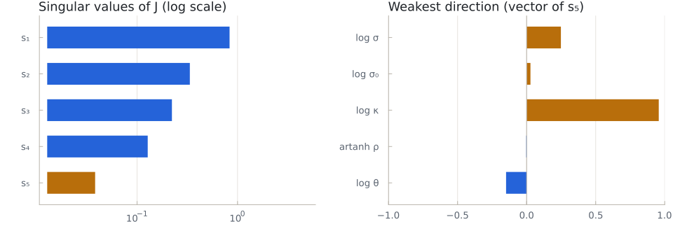

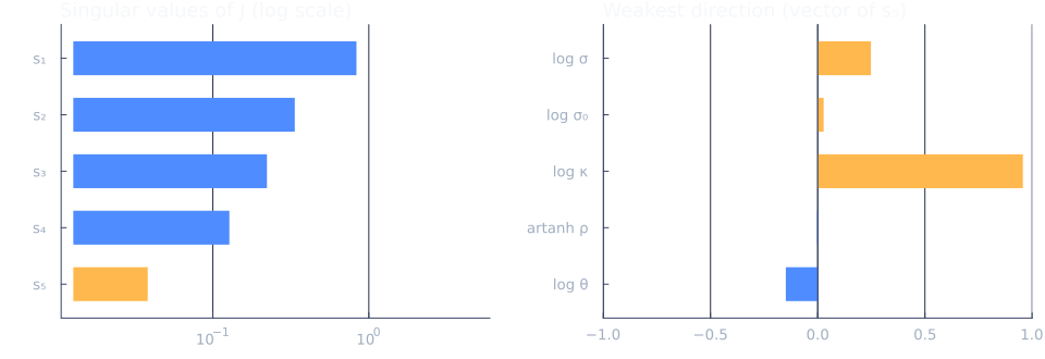
The weakest direction, in the variables $x = (\log \sigma, \log \sigma_0, \log \kappa, \operatorname{artanh} \rho, \log \theta)$, is mostly $\log \kappa$, with the volatility of the variance and the level $\theta$ compensating it: the speed of mean reversion shows only in how the smile changes with the maturity, and four maturities up to two years see it weakly.

Sensitivity of the calibrated parameters to the quotes

How do the calibrated parameters $x^*$ move when a quote moves? The implicit function theorem gives the derivatives of the calibration without differentiating the optimizer. At the optimum the gradient of the loss vanishes,

\[g(x^*, v) = \partial_x L(x^*, v) = J^\top e(x^*) = 0,\]

and where $\partial_x g$ is invertible

\[\frac{\partial x^*}{\partial v} = -\left(\partial_x g\right)^{-1} \partial_v g = H^{-1} J^\top, \qquad H = \partial^2_x L = J^\top J + \sum_{i=1}^n e_i \, \partial^2_x e_i ,\]

since $\partial_v g = -J^\top$. The FinancialFFT page computes $H$, $J$ and the product by hand. Here calibrated_parameters is the calibration as a function of the quoted volatilities, with these derivatives as its rules (ImplicitDifferentiation.jl builds them from the solver and the conditions $g = 0$): a method for ForwardDiff's dual numbers and a ChainRules reverse rule. The whole $6 \times n$ Jacobian is one call:

∂p_∂v = ForwardDiff.jacobian(w -> calibrated_parameters(start, method, mkt, w; parametrization = variables, min_vega = 0), vols)
size(∂p_∂v)

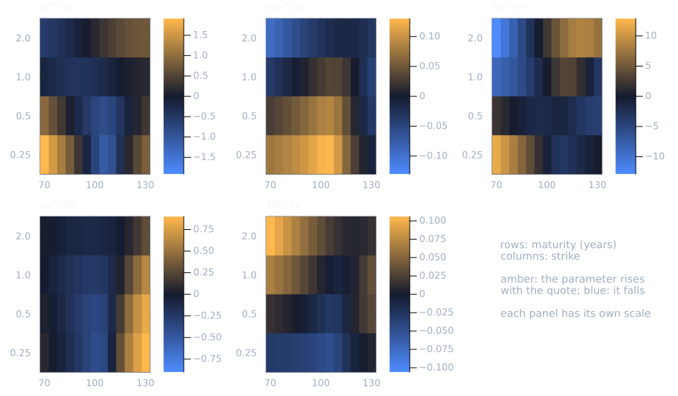
(6, 52)

Its columns follow the entries of vols (column major: maturity first). Row by row, on the grid of the quotes:

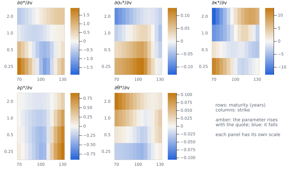
The quoted volatilities depend on the prices through the inverse of the vega, $\partial v_i / \partial m_i = 1 / \nu_i$, so the sensitivities to the quoted prices are

\[\frac{\partial p^*}{\partial m} = \frac{\partial p^*}{\partial v} \operatorname{diag}\left(\frac{1}{\nu_1}, \dots, \frac{1}{\nu_n}\right).\]

A check on one quote, the put with strike 85 at one year, against moving its volatility by a basis point both ways and recalibrating:

i = CartesianIndex(3, 4)
bump(h) = (w = copy(vols); w[i] += h; w)
recalibrate(h) = calibrated_parameters(start, method, mkt, bump(h); parametrization = variables, min_vega = 0)
h = 1e-4
(implicit = ∂p_∂v[:, LinearIndices(vols)[i]], recalibrated = (recalibrate(h) - recalibrate(-h)) / 2h)

(implicit = [-0.39584068596379507, -0.0042681013621352504, 0.0, -5.486060625246376, -0.16814137778351496, 0.040256737818743275], recalibrated = [-0.3958406849272067, -0.0042681024121915545, 0.0, -5.4860607074136425, -0.1681413740484139, 0.04025673891194098])

The implicit derivatives match the recalibration to the accuracy of the finite difference, and cost one solve and one pass of dual numbers instead of two calibrations per quote. The parameters $\lambda$ (row 3), which the parametrization fixes, have no sensitivity.