Guide 02 Three independent choices
Methods, backends and arrays
A calibration combines three choices that the package keeps independent: how a smile is priced, how derivatives are taken, and where the arrays live. Each one is an argument, and changing one does not change the others.
How a smile is priced
Fourier for Lévy models and Heston, a closed form where one exists, Monte Carlo for everything else.
Default pick LewisMethod; CosMethod where its series converges (Heston, Black–Scholes).
How derivatives are taken
Outside the calibration any backend; inside, four keywords, each an ADTypes backend.
Default pick ForwardDiff everywhere; a reverse backend outside with many quotes.
03 · ArraysWhere the numbers live
Float64 or Float32, on the host or on a CUDA device, derivatives included.
Default pick the CPU for a surface of a hundred quotes; the GPU for large smiles.
Pricing methods
The second argument of calibrate is any pricing method of FinancialMonteCarlo's pricer interface, so the kind of calibration is the choice of that argument:
| Method | Package | Models |
|---|---|---|
LewisMethod, CosMethod, CarrMadanLewisMethod, CarrMadanMethod | FinancialFFT.jl | every model with a characteristic exponent: Black–Scholes, Merton, Kou, Variance Gamma, NIG, Heston |
AnalyticMethod | FinancialCalibrator.jl | closed forms: BlackScholesProcess, ShiftedLogNormalMixture, see Closed forms |
MonteCarloConfiguration | FinancialMonteCarlo.jl | every model that it simulates, with the same seed at every evaluation |
Vibrato, VibratoSaltando, PureLRM | VibratoMonteCarlo.jl | Monte Carlo with smooth estimators of the derivatives |
calibrate(model, CosMethod(2^10), mkt)                                   # Fourier
calibrate(model, LewisMethod(400.0, 40001), mkt)                         # Fourier, another quadrature
calibrate(slnm, AnalyticMethod(), mkt)                                   # closed form
calibrate(model, MonteCarloConfiguration(10^5, 1), mkt)                  # simulation
The same Heston calibration of the DAX surface with three Fourier methods (measured by docs/benchmarks.jl):
| Heston, DAX, pricing engine | one loss | calibration | RMS error |
|---|---|---|---|
CosMethod(2^10) | 3.68 ms | 763 ms | 68.9 bp |
LewisMethod(100, 4001) | 6.65 ms | 1.58 s | 68.9 bp |
CarrMadanLewisMethod(600, 16) | 251.42 ms | 51.46 s | 68.9 bp |
Same model, same optimum: the engine sets the cost. CarrMadanLewisMethod(600, 16) runs an FFT of 2¹⁶ points per maturity, far more than nine smiles of twelve strikes need.
A new model and method pair needs only a pricer method for a smile. The model is any FinancialMonteCarlo process; the parameters the calibration moves are those of FinancialMonteCarlo.get_parameters, or the variables of a Parametrization.
The derivatives of the calibration (the Levenberg–Marquardt polish and calibrated_parameters) need a method whose derivatives are those of its prices. FinancialFFT's methods differentiate their quadrature exactly; the truncation range of CosMethod is held constant, which matters only where its series has not converged (Variance Gamma and NIG at short maturities, see FinancialFFT.jl#64). A Monte Carlo method gives the pathwise derivative of its estimator on its fixed paths.
Automatic differentiation
From outside
calibrated_parameters is a function of the quoted volatilities that every backend can differentiate, since its rules come from the implicit function theorem and not from tracing the optimizer:
using ForwardDiff, Zygote
f(v) = calibrated_parameters(model, method, mkt, v)
ForwardDiff.jacobian(f, mkt.Volatility)                    # ∂p*/∂v, forward mode
Zygote.gradient(v -> w' * f(v), mkt.Volatility)            # wᵀ ∂p*/∂v, reverse mode (ChainRules)
Mooncake has a rule of its own, in the package extension loaded with Mooncake (ImplicitDifferentiation's ChainRules rule needs a RuleConfig, which Mooncake.@from_rrule does not pass):
using Mooncake, ADTypes
import DifferentiationInterface as DI
DI.gradient(v -> w' * f(v), AutoMooncake(; config = nothing), mkt.Volatility)
Support
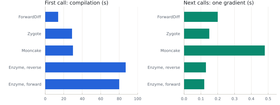
Every derivative of the calibration runs through the implicit function theorem, so the outer backend never traces the optimizer: it only meets the rule of the implicit function, and the inner backends meet the loss. The backends can be mixed freely, forward over reverse or reverse over forward. The table shows the gradient of $w^\top p^*(v)$ for Variance Gamma with LewisMethod(100.0, 4001) on 15 quotes, relative to the ForwardDiff gradient on the host. Every case ran in a fresh Julia process. The first call is timed after one calibration in that process, so it is the compilation of the derivatives only; the device is a laptop GPU (NVIDIA MX150):
| Outer | Inner x / y | Host: first call | Host: next calls | Device: next calls | Error |
|---|---|---|---|---|---|
| ForwardDiff¹ | ForwardDiff / ForwardDiff | 14 s | 0.20 s | 0.32 s² | 0 (host), 5e-13 (device) |
| Zygote | ForwardDiff / ForwardDiff | 29 s | 0.15 s | 0.38 s | 2e-14, 2e-12 |
| Mooncake | ForwardDiff / ForwardDiff | 30 s | 0.48 s | 0.74 s | 2e-14, 2e-12 |
| Zygote | Mooncake / ForwardDiff | 138 s | 0.71 s | ✗³ | 2e-14 |
| Mooncake | Mooncake / ForwardDiff | 127 s | 0.41 s | ✗³ | 2e-14 |
| Enzyme, reverse⁴ | ForwardDiff / ForwardDiff | 87 s | 0.13 s | 0.43 s | 2e-14, 2e-12 |
| Enzyme, forward⁴ | ForwardDiff / ForwardDiff | 80 s | 0.12 s | ✗⁵ | 1e-15 |
One run per case: on this laptop the times of two runs differ by up to a third.
¹ With one chunk for all the quotes, ForwardDiff.gradient(f, v, ForwardDiff.GradientConfig(f, v, ForwardDiff.Chunk{length(v)}())). ForwardDiff's default chunk (8) splits 15 quotes in two, and each chunk runs the whole calibration again. ² One direction: ForwardDiff cannot seed a CuArray, so on the device it gives one derivative at a time (ForwardDiff.derivative along a bump of one quote). ³ Mooncake differentiating the inner ForwardDiff gradient of the conditions meets a broadcast of dual numbers over a CuArray, which it does not support. ⁴ Enzyme works through rules of the extension of FinancialCalibrator for EnzymeCore: they build the implicit function outside of the differentiated code, then apply ImplicitDifferentiation's Enzyme rules to it as a constant (Enzyme cannot trace the construction, and failed on the GPU when it did, #21). Those rules need the solver to return an inferred type, which it does. On the device the first call compiles for 4 to 7 minutes here, 18 on Black–Scholes with CosMethod(1024). ⁵ Enzyme's forward mode seeds the gradient with one-hot arrays that it fills by scalar indexing, which a CuArray refuses (EnzymeAD/Enzyme.jl#4048); the reverse mode works on the device.
What the numbers say:
- Once compiled, a gradient costs about one calibration, whatever the backend: here the solve takes 0.1 to 0.2 s (NelderMead, then the Levenberg–Marquardt polish), and the derivatives of the implicit function theorem about 8 ms. Reverse mode outside pays off with many quotes, not with these 15.
- The first call is compilation: Zygote and Mooncake compile their rules for the whole pricing method.
- A reverse backend for
xis reverse over forward: Mooncake differentiates the ForwardDiff gradient of the loss, through the pricer. That compiles for minutes and runs 5 times slower than ForwardDiff forx; it can pay off only with many quotes, where forward mode needs one direction per quote.
The test suite checks ForwardDiff, Zygote, Mooncake and Enzyme (reverse, and forward on Black–Scholes) against the formula $\partial p^*/\partial v = -H^{-1} \partial_v \nabla_p L$, and Zygote and Mooncake on the GPU.
Inside
Four derivatives are taken inside, each by an ADTypes.jl backend, through DifferentiationInterface.jl:
| Keyword | Of | Default |
|---|---|---|
autodiff | the gradient of the loss, for a gradient based Optim optimizer (LBFGS(), BFGS(), ...) | AutoForwardDiff() |
polish_backend | the Jacobian $J$ of the volatility errors, in the Levenberg–Marquardt polish | AutoForwardDiff() |
conditions_backend | the gradient $g = \partial_x L$, the optimality conditions | AutoForwardDiff() |
implicit_backends = (x = ..., y = ...) | the derivatives of $g$ with respect to the quotes (x) and to the variables (y) | AutoForwardDiff() for both |
The last row differentiates the gradient of the row before it: a second order derivative, nested. ForwardDiff everywhere suits a calibration, whose parameters are few: the Jacobian $J$ has as many columns as parameters, and the Hessian $\partial_x g$ is small. The one place where reverse mode can pay is x with a reverse outer backend and many quotes: the reverse rule needs $(\partial_v g)^\top w$, which forward mode gets one quote at a time.
using ADTypes, Mooncake
calibrated_parameters(model, method, mkt, v; implicit_backends = (x = AutoMooncake(; config = nothing), y = AutoForwardDiff()))
The table above times these combinations. Zygote for x does not work: it cannot differentiate the inner ForwardDiff gradient of the conditions.
Arrays
Floating point types
MarketData and CalibratedData are parametric in the floating point type. adapter(raw, Float32) reads a surface in Float32, and the losses are computed in it.
GPU
The strikes and the volatilities of MarketData can live on the GPU. With CUDA.jl loaded, every smile is then priced on the device (the extension moves the method to CudaMode), the implied volatilities are a broadcast on the device, and so are the derivatives: the dual numbers of ForwardDiff and the cotangents of Zygote are CuArrays too. The small linear systems (the Levenberg–Marquardt step, the implicit function theorem) come back to the CPU.
using CUDA, Adapt
gmkt = adapt(CuArray, mkt)                                            # strikes and volatilities on the device
calibrate(model, CosMethod(1024), gmkt)
calibrated_parameters(model, CosMethod(1024), gmkt)
Zygote.gradient(V -> sum(calibrated_parameters(model, CosMethod(1024), gmkt, V)), gmkt.Volatility)[1]   # a CuMatrix
Measured on a laptop GPU (NVIDIA MX150) with the DAX surface of 108 quotes, once compiled:
| Host | Device | Agreement | |
|---|---|---|---|
calibrate, Black–Scholes, CosMethod(1024) | 0.06 s | 0.41 s | 4e-15 |
calibrate, Variance Gamma, LewisMethod(100.0, 4001) | 0.36 s | 0.71 s | 3e-8 |
one loss, Black–Scholes, CosMethod(1024) | 1.1 ms | 8.5 ms | |
one loss, Variance Gamma, LewisMethod(100.0, 4001) | 2.7 ms | 7.2 ms | |
| Zygote gradient, Black–Scholes | 4e-14 | ||
| Zygote gradient, Variance Gamma | 8e-8 |
How the cost of one loss grows with the strikes of a smile, on the same laptop (Black–Scholes, CosMethod(4096), measured by docs/benchmarks.jl):
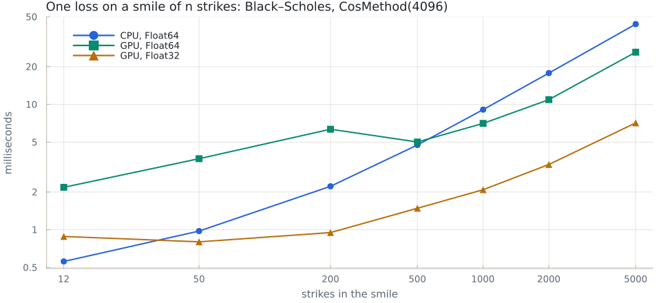
A smile of 12 strikes is far too small to occupy a GPU, and these numbers time kernel launches: a loss costs 7 to 9 ms on the device whatever the model and the method. The device pays off with many strikes per smile, or many quotes. The point here is that nothing in the calibration, nor in its derivatives, needs to leave the device.
Float32
Consumer GPUs compute in Float64 at a fraction of their Float32 rate (1/32 on the MX150), and adapter(raw, Float32) gives a surface in Float32. On the DAX surface this changes nothing on the device, since the launches dominate: a loss costs 9.1 ms (Black–Scholes, Cos) and 7.6 ms (Variance Gamma, Lewis), and a calibration takes about as long (Black–Scholes 0.46 s, Variance Gamma 0.75 s, parameters within 2e-4 of the host in Float32). On a smile large enough to occupy the device, Float32 pays: 2000 strikes with CosMethod(4096):
| Host | Device | |
|---|---|---|
Float64 | 17.7 ms | 14.3 ms |
Float32 | 17.6 ms | 6.7 ms |