FinancialCalibrator.jl

Differentiable Calibration of Option Pricing Models

Calibrate volatility surfaces, compute sensitivities, and obtain quote-to-risk derivatives through automatic differentiation in Julia.

res   = calibrate(model, method, mkt)            # p*
p(v)  = calibrated_parameters(model, method, mkt, v)
∂p_∂v = ForwardDiff.jacobian(p, mkt.Volatility) # ∂p*/∂v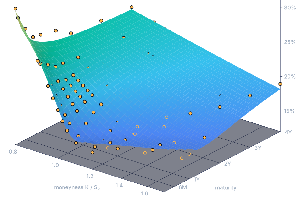

Implied volatility surface of a Heston model calibrated to the DAX, with the market quotes as dots — DAX quote left out of the loss (low vega) calibrated Heston surface, coloured by implied volatility Heston calibrated to the DAX surface of 22 August 2016, rendered from the package's output when this site was built.

69 bp

RMS volatility error, Heston on 99 DAX quotes

0.75 s

to calibrate it with LBFGS + Levenberg–Marquardt, on a laptop CPU

6 × 108

Jacobian ∂p*/∂v from one ForwardDiff call

AD backends through the calibration: ForwardDiff, Zygote, Mooncake, Enzyme

What it does

Most calibrators return a point estimate. FinancialCalibrator.jl returns the calibrated parameters as a differentiable function of the quotes: the derivatives come from the implicit function theorem at the optimum, never from unrolling the optimizer, so every risk number downstream of the calibration is one gradient away.

Differentiable calibration

calibrated_parameters is the calibration as a function of the quoted volatilities, with its own derivative rules.

Sensitivities without bump-and-recalibrate: one call instead of two calibrations per quote.

Quote-to-risk sensitivities

The derivative of any contract priced with the calibrated model, an exotic or a whole position, with respect to every quote of the surface.

Bucketed vega that is consistent with the model you price with, from a single gradient.

Multiple pricing engines

Fourier (Lewis, COS, Carr–Madan), closed forms, Monte Carlo and Vibrato Monte Carlo, through one pricer interface.

Change the engine with one argument; speed and generality become a choice, not a rewrite.

GPU acceleration

Strikes and quotes as CuArrays: pricing, implied volatilities and derivatives stay on the device, in Float64 or Float32.

6× the CPU in Float32 on a 5000-strike smile, on a laptop GPU; a small surface is launch-bound.

Implicit differentiation

At the optimum ∇L = 0, so ∂x*/∂v = H⁻¹Jᵀ: the derivative needs the conditions, not the path of the optimizer.

Matches −H⁻¹∂ᵥ∇L to 1e-14 in the tests; about 8 ms on top of the solve.

Multiple AD backends

ForwardDiff, Zygote, Mooncake and Enzyme outside; any ADTypes backend inside, mixed freely. None is a hard dependency.

Use the backend your pipeline already uses; forward for few quotes, reverse for many.

Extensible model framework

Any FinancialMonteCarlo process: Black–Scholes, Merton, Kou, VG, NIG, Heston, lognormal mixtures. A new model–method pair is one pricer method.

Parametrization handles constraints and fixed parameters, so no step yields an invalid model.

Production-ready workflows

Out-of-the-money quotes filtered by vega, a Levenberg–Marquardt polish to a stationary point (|∇L| ~ 1e-8), Inf for unpriceable parameters, CBOE data loader.

Tested against recalibration and against a hand-written reference calibration.

How it fits together

Quotes flow left to right into risk; derivatives flow back along the same path. Each box is one function call, and each arrow is differentiable.

01Market quotesCBOE delayed quotes, JSON snapshots
retriever
02Volatility surfaceOTM vols, rates, implied dividends
adapter → MarketData
03FinancialCalibrator.jlOptim + Levenberg–Marquardt; implicit function theorem
calibrate, calibrated_parameters
04Calibrated parametersp*(v), with ∂p*/∂v
Parametrization
05Pricing enginesFinancialFFT, closed form, Monte Carlo
pricer
06Risk sensitivities∂V/∂vᵢ for every quote
one gradient

∂V/∂v = ∇ₚV(p*)ᵀ · ∂p*/∂v ← chain rule through the pricer, then the implicit function theorem through the calibration

Results on a real surface

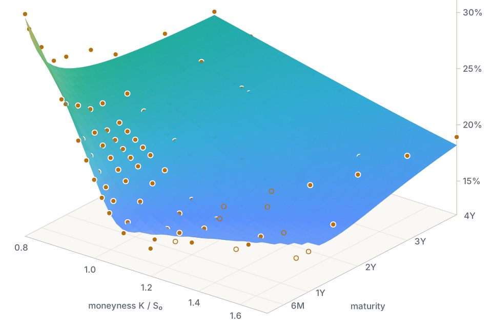
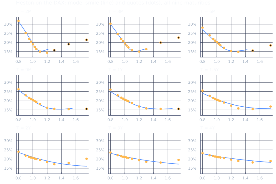
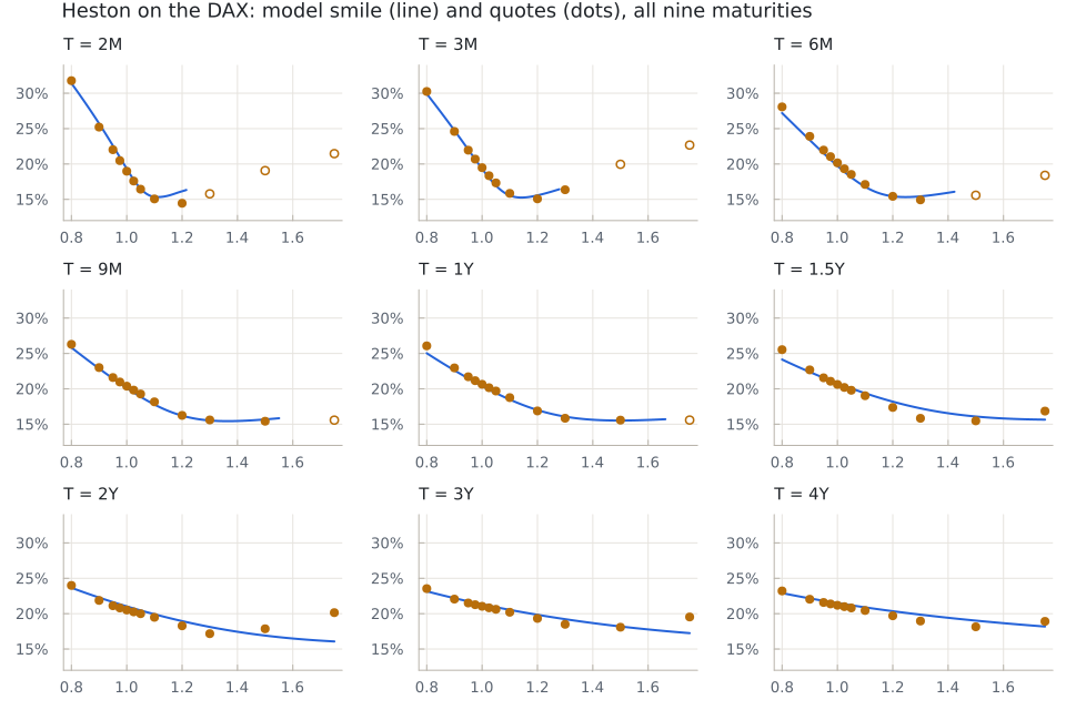
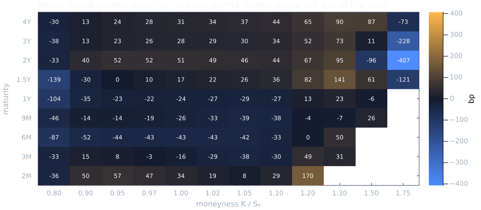
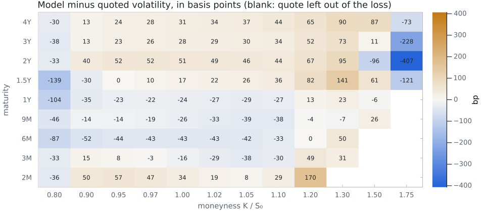
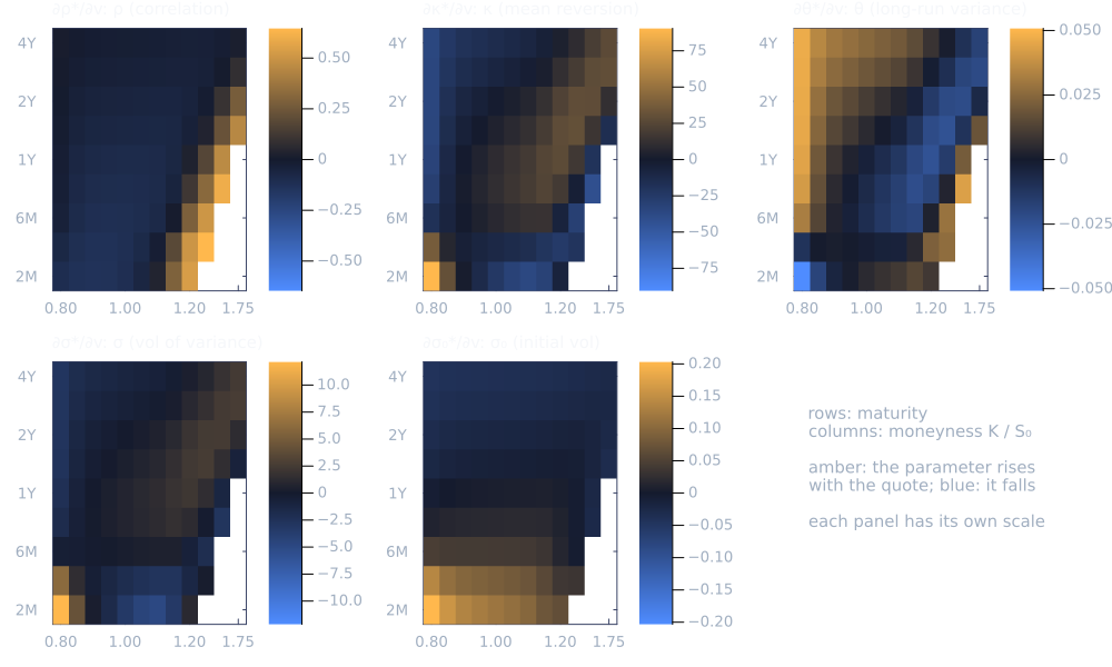
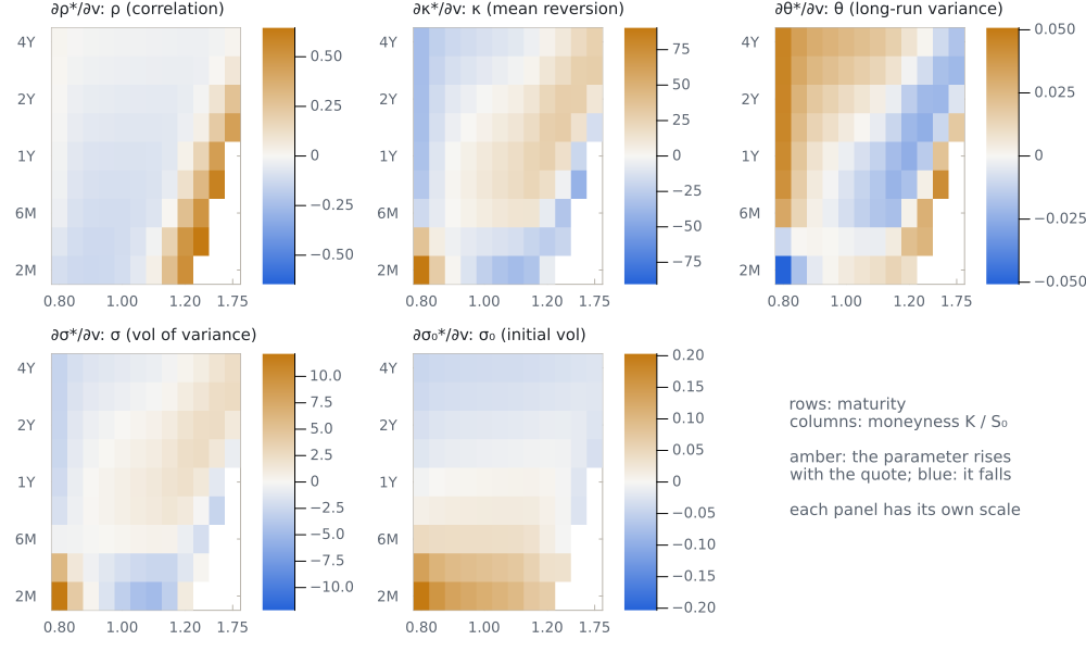
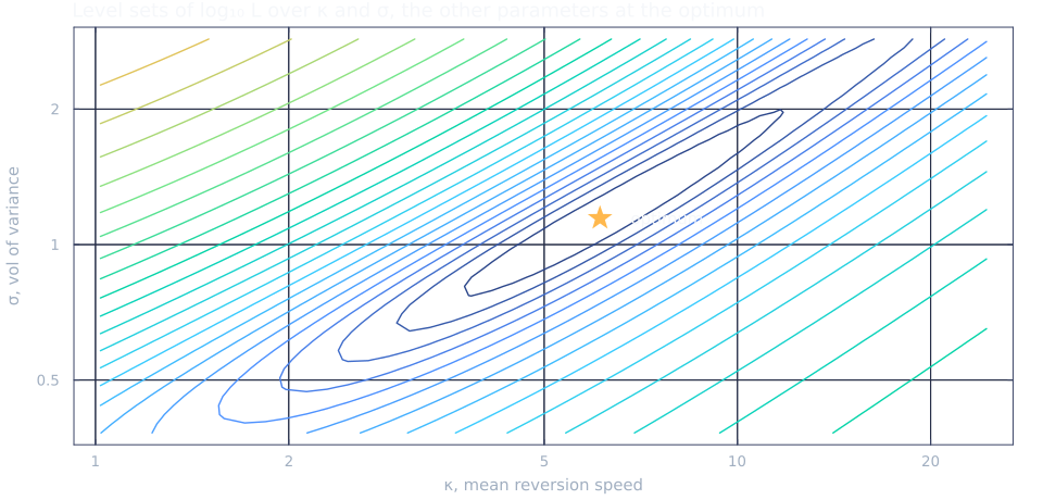
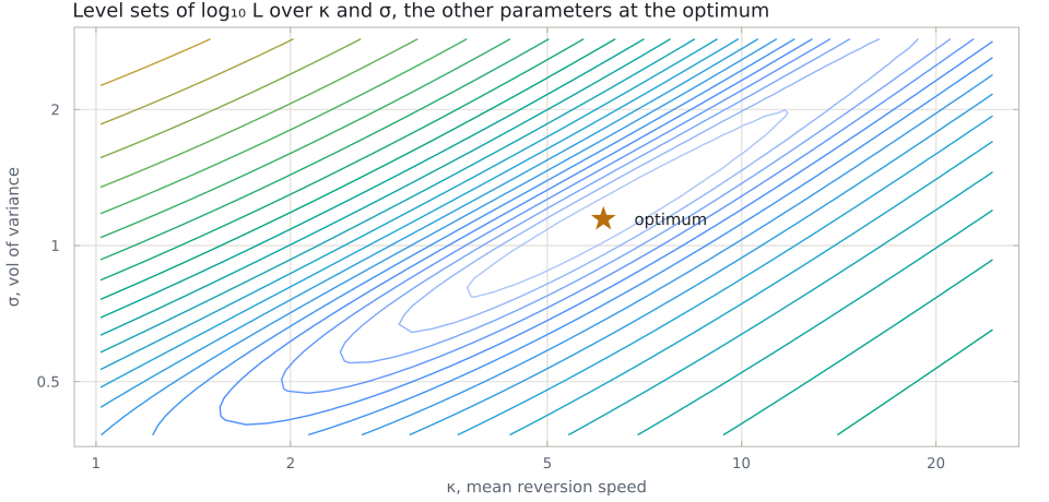
Computed by the package when this site is built, from the DAX surface that ships with it: 9 maturities from two months to four years, 12 strikes from 0.8 to 1.75 times the spot.

Smiles Errors Parameter sensitivities Loss landscape

Model smiles and quotes for the nine maturities — **The smile at every maturity.** Closest around the money; the far wings are where one Heston model gives way.

Heatmap of model minus market volatility in basis points — **Where the error is.** Model minus quoted volatility, in bp; the 9 quotes with too little vega are blank.

Heatmaps of the sensitivity of each Heston parameter to each quote — **Which quotes move which parameter.** ∂p*/∂v from one ForwardDiff call: ρ follows the right wing, σ₀ the short end; κ is the weakest direction.

Contour lines of the loss over kappa and sigma — **The landscape the optimizer sees.** The long valley in (κ, σ) is why κ is hard to pin down, and why the polish to a stationary point matters.

Benchmarks

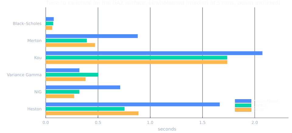
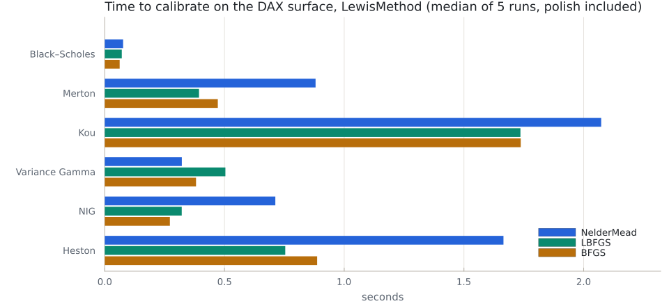
Measured on a laptop CPU and GPU, medians after compilation: which choice to make, not a headline number. Scaling, AD backends and pricing engines in detail: Methods, backends and arrays.

754 ms

Heston on 99 DAX quotes with LBFGS: 2.2× faster than Nelder–Mead, same optimum (68.9 bp)

≈ 1 calibration

the cost of a full gradient ∂p*/∂v once compiled: the implicit derivatives themselves take ~8 ms

6.1×

GPU in Float32 over the CPU, one loss on a smile of 5000 strikes (NVIDIA GeForce MX150); in Float64 the GPU overtakes the CPU near 500 strikes

14 s

first-call compilation with ForwardDiff outside; 29–30 s Zygote or Mooncake, 80–90 s Enzyme

Measured 2026-11-13 on Intel(R) Core(TM) i7-8550U CPU @ 1.80GHz, 1 thread(s), Julia 1.13.3, GPU NVIDIA GeForce MX150. Script: docs/benchmarks.jl; raw data: docs/src/assets/benchmarks.toml.

Optimizers

Every optimizer ends at the same optimum: the Levenberg–Marquardt polish takes over from wherever it stops. Insight: pass LBFGS() or BFGS() for Heston, Merton and NIG, 2 to 2.6× faster than the default Nelder–Mead.

Calibration time per model and optimizer

Use cases

built in works out of the box; compose is built on top of it with the rest of the Julia ecosystem.

Equity volatility

built in

Fit Heston or a Lévy model to an index surface from DAX or CBOE data.

A stationary optimum and its error in bp, in about a second.

Exotic-option pricing

built in

Price American, Asian, barrier payoffs consistently with the vanillas.

A price and its vega to every quote, through simulation and calibration.

Risk management

built in

Bucketed vega of a book on a model that would need a recalibration per bump.

The whole sensitivity surface for about one calibration.

Model validation

built in

Are the parameters identified by the quotes? Is the optimum a true one?

Weak directions from the singular values of J, |∇L| at the optimum.

Differentiable research

built in

A calibration inside an objective: a bilevel problem.

Exact gradients of the outer objective, no unrolled optimizer.

FX volatility

compose

Delta quotes converted to strikes; the foreign rate as the dividend yield.

The same calibration and sensitivities as for equity.

Commodity derivatives

compose

One smile per futures expiry; the cost of carry as the dividend curve.

Parameters and their sensitivity to each quoted vol.

ML-assisted calibration

compose

calibrated_parameters as a differentiable layer in a training loop.

Gradients that respect the calibration exactly, CPU or GPU.

Quick start

Six steps, two minutes, a real surface. Every output below was produced by this code when the site was built.

Install the package

FinancialFFT.jl is in a registry of its own, added once.

] registry add https://github.com/rcalxrc08/LocalRegistry.git
] add https://github.com/rcalxrc08/FinancialCalibrator.jl
] add FinancialMonteCarlo, FinancialFFT, ForwardDiff

Load market data

The bundled DAX surface, as the underlying and the MarketData of the calibration.

using FinancialCalibrator, FinancialMonteCarlo, FinancialFFT, ForwardDiff

und, mkt = adapter(retriever(CalibrationID("Dax", "22Aug2016", "EUR"), IOFileInputStrategy()))
size(mkt.Volatility)   # maturities × strikes

(9, 12)

Build a calibration problem

A model at its starting point, and a pricing engine.

model = NormalInverseGaussianProcess(0.2, -0.03, 0.16, und)   # σ, θ, κ: the starting point
method = LewisMethod(100.0, 4001)

Run the calibration

Nelder–Mead by default, then a Levenberg–Marquardt polish to a stationary point.

res = calibrate(model, method, mkt)
res.OptimalParam

3-element Vector{Float64}:
  0.15967036960214767
 -0.31502283136966547
  0.2667616330152099

Compute sensitivities

∂p*/∂v for all 108 quotes, by the implicit function theorem.

∂p_∂v = ForwardDiff.jacobian(v -> calibrated_parameters(model, method, mkt, v), mkt.Volatility)
size(∂p_∂v)   # parameters × quotes

(3, 108)

Analyse the results

The fit in bp, the worst quote, and the response to a parallel shift.

e = 1e4 .* (res.ModelVolatility .- mkt.Volatility)       # errors in bp, NaN where left out
worst = argmax(i -> isnan(e[i]) ? -Inf : abs(e[i]), CartesianIndices(e))
(rms_bp = round(sqrt(sum(abs2, filter(!isnan, e)) / count(!isnan, e)); digits = 1),
 worst_quote = (T = mkt.TimeToMaturity[worst[1]], moneyness = round(mkt.Strikes[worst[2]] / und.S0; digits = 2), error_bp = round(e[worst]; digits = 1)),
 parallel_shift = round.(vec(sum(∂p_∂v; dims = 2)); digits = 3))   # ∂p*/∂h for every quote moved by h

(rms_bp = 86.7, worst_quote = (T = 2.0, moneyness = 1.75, error_bp = -326.0), parallel_shift = [1.057, -0.909, 0.365])

Calibration, step by stepThe loss, the polish, identifiability and the implicit derivatives, on Heston. Methods, backends and arraysPricing engines, AD backends inside and out, GPU and Float32. Sensitivities of exoticsMonte Carlo positions and their vega to every quote. API referenceEvery exported function and type.

The ecosystem

FinancialMonteCarlo.jl defines the models, the payoffs and the pricer interface, FinancialFFT.jl the Fourier pricing methods, and FinancialToolbox.jl the implied volatility blsimpv. FinancialCalibrator.jl adds the loss, the optimization and the derivatives of the calibration. Market data comes from the bundled DAX surface or from the free delayed quotes of the CBOE, see Market data. More projects at rcalxrc08.github.io.