Guide 03 Exact prices, no numerical method
Closed forms: the shifted lognormal mixture
AnalyticMethod prices
a smile with the closed form of the model, when it has one: Black and Scholes, and the shifted lognormal
mixture of Brigo and Mercurio. The second is a model worth calibrating on its own, and this page is about
it.
The model
The spot is a deterministic shift plus a process $A$ whose law at each time is a mixture of lognormals:
\[S_t = \alpha\, S_0\, e^{(r - d) t} + A_t, \qquad A_0 = (1 - \alpha) S_0, \qquad A_T \sim \sum_{j=1}^{n} w_j\, A_0\, e^{(r - d - \eta_j^2 / 2) T + \eta_j \sqrt{T} Z},\]
with $Z$ standard normal, volatilities $\eta_1, \dots, \eta_n > 0$ and weights $w_j = \lambda_j$ for $j < n$, $w_n = 1 - \sum_{j<n} \lambda_j$. ShiftedLogNormalMixture(η, λ, α, underlying) takes the $n$ volatilities, the $n - 1$ free weights and the shift $\alpha < 1$. Brigo and Mercurio show that a local volatility $\sigma(t, A_t)$ exists for which $A$ has exactly these marginals: the model is a diffusion, and not only a family of densities. FinancialMonteCarlo's simulation of ShiftedLogNormalMixture is not that diffusion (it sums the lognormal processes path by path, a model with other European prices, see FinancialMonteCarlo.jl#56): do not price exotics by Monte Carlo with a model calibrated by its closed form until that is settled.
A European option on $S$ is an option on $A$ struck at $\kappa = K - \alpha S_0 e^{(r - d) T}$, and the mixture passes through the expectation: its price is the mixture of Black prices,
\[C(K, T) = \sum_{j=1}^{n} w_j\, C_{\text{black}}\!\left((1 - \alpha) F_T, \kappa, r, T, \eta_j\right), \qquad F_T = S_0 e^{(r - d) T},\]
and the same for a put. For $\kappa \le 0$ (a positive shift and a strike below it) the call is always exercised, $C = e^{-rT}(F_T - K)$, and the put is worthless. The implementation computes the shift, the forward and the weights once per smile, then one Black price per component and strike, by blkprice of FinancialToolbox.
Why calibrate it
A price is n Black formulas: no quadrature, no truncation range, no simulation. A smile of a few hundred strikes with three components prices in about 0.15 ms on a laptop. The loss has no numerical noise, so the optimizer and the Levenberg–Marquardt polish reach a stationary point to machine precision, and the implicit derivatives of calibrated_parameters are those of the exact calibration.
A mixture of arbitrage-free prices is arbitrage free: the prices are decreasing and convex in the strike, and the forward is matched exactly, for every parameter, so no constraint is needed beyond the signs of η and λ.
The mixture gives fat tails, the smile: the volatilities η are the regimes, the weights how likely they are. The shift gives the skew: α < 0 makes the spot more lognormal than A, with a downward sloping implied volatility; α > 0 the opposite.
The formula is a broadcast of blkprice, which has closed-form ChainRules rules: ForwardDiff, Zygote and Mooncake differentiate it as well as the Fourier methods.
The components are a tuple whose length is a type parameter, so a smile is one broadcast over its strikes, one thread per strike. With the strikes of MarketData on the device, or AnalyticMethod(; mode = CudaMode()), the prices never leave it.
Its limit is the term structure. The parameters are the same at every maturity, and the smile of a mixture of lognormals flattens with the maturity as $1/\sqrt{T}$ in log-moneyness: one set of parameters fits a few maturities, or one maturity at a time, better than a whole surface. Its local volatility dynamics also give forward smiles that are flatter than the market's, which matters for forward starting and cliquet options, not for the European quotes it is calibrated to.
On the DAX surface
The DAX surface of 22 August 2016, with three components, against Black and Scholes (a single component and no shift), both with the closed form:
using FinancialCalibrator, FinancialMonteCarlo

underlying, mkt = adapter(retriever(CalibrationID("Dax", "22Aug2016", "EUR"), IOFileInputStrategy()))
rms(res) = sqrt(2 * res.OptimalValue / count(!isnan, res.ModelVolatility))

bs = calibrate(BlackScholesProcess(0.2, underlying), AnalyticMethod(), mkt)
slnm = calibrate(ShiftedLogNormalMixture([0.1, 0.2, 0.35], [0.3, 0.4], -0.1, underlying), AnalyticMethod(), mkt)
(black_scholes = rms(bs), shifted_lognormal_mixture = rms(slnm))
(black_scholes = 0.0315196877737609, shifted_lognormal_mixture = 0.021199392732466515)Four of the nine maturities, the model volatilities at the quotes:
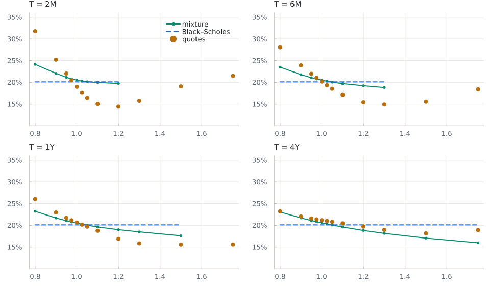
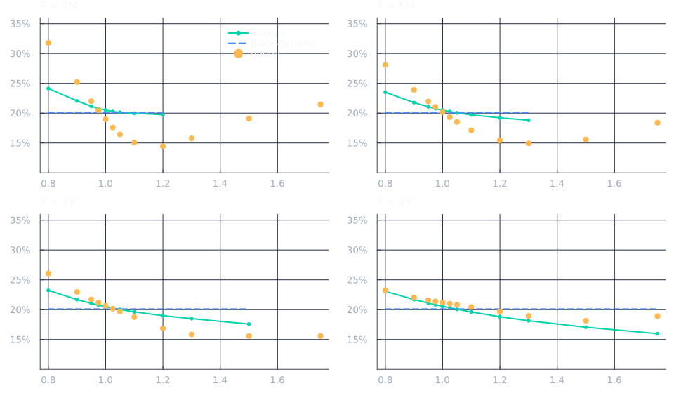
The calibrated parameters, $(\eta_1, \eta_2, \eta_3, \lambda_1, \lambda_2, \alpha)$:
slnm.OptimalParam6-element Vector{Float64}:
0.0009573793790001189
2.089198834093455e-36
0.0006121626134154711
0.7556752777184548
2.2262104523350895e-55
-233.71401490820045Other closed forms
A model gets a closed form by two methods, FinancialCalibrator.analytic_price_type(model) (the number type of its prices) and FinancialCalibrator.analytic_kernel(model, S0, r, d, T) (a callable (K, isCall) -> price, an isbits struct so that a GPU broadcast captures it); pricer(model, zero_rate, AnalyticMethod(), smile) does the rest, on the host or on the device.