Sensitivities of exotics to the surface

\[V^*(v) = V\big(p^*(v)\big), \qquad \frac{\partial V^*}{\partial v_i} = \nabla_p V\big(p^*\big)^\top \frac{\partial p^*}{\partial v_i} .\]

$\partial p^* / \partial v$ comes from the implicit function theorem (see Calibration), and $\nabla_p V$ from automatic differentiation through the pricer of the contract. Since calibrated_parameters carries the rules of the first factor, both are one gradient of the composition, with no matrix assembled by hand.

The calibrated model

The Heston calibration of the Calibration page, on the same quotes:

using FinancialCalibrator, FinancialMonteCarlo, FinancialFFT, FinancialToolbox, ForwardDiff, Dates

S0, r, d = 100.0, 0.02, 0.01
zero_rate = ZeroRate(r)
underlying = Underlying(S0, d)
maturities = [0.25, 0.5, 1.0, 2.0]
strikes = collect(70.0:5.0:130.0)
method = CosMethod(2^9)
heston_market = HestonProcess(0.5, 0.2, 0.0, 1.5, -0.7, 0.04, underlying)
function quoted_vols(T, row)
    calls = strikes .>= S0 * exp((r - d) * T)
    prices = pricer(heston_market, zero_rate, method, FinancialMonteCarlo.EuropeanOptionSmile(T, strikes, calls))
    prices = prices .* (1 .+ 0.01 .* sin.((row - 1) * length(strikes) .+ (1:length(strikes))))
    return blsimpv.(S0, strikes, r, T, prices, d, calls)
end
vols = reduce(vcat, [permutedims(quoted_vols(T, i)) for (i, T) in enumerate(maturities)])
mkt = MarketData(maturities, [Date(2026) + Day(round(Int, 365 * T)) for T in maturities], fill(r, length(maturities)), strikes, vols)
variables = Parametrization(x -> [exp(x[1]), exp(x[2]), zero(x[1]), exp(x[3]), tanh(x[4]), exp(x[5])],
                            p -> [log(p[1]), log(p[2]), log(p[4]), atanh(p[5]), log(p[6])])
start = HestonProcess(0.3, 0.25, 0.0, 1.0, -0.3, 0.06, underlying)
calibrated(w) = calibrated_parameters(start, method, mkt, w; parametrization = variables, min_vega = 0)

A position, priced by Monte Carlo

FinancialMonteCarlo simulates the calibrated Heston and prices any of its payoffs, alone or combined into a position with +, - and *. The position here is long an American put (strike 95, one year, Longstaff–Schwartz), short half an Asian call (strike 100, one year, arithmetic average on the simulation dates) and long two European calls with a maturity that no quote has (strike 110, eighteen months):

position = AmericanOption(1.0, 95.0, false) - 0.5 * AsianFixedStrikeOption(1.0, 100.0) + 2 * EuropeanOption(1.5, 110.0)
mc = MonteCarloConfiguration(20_000, 50)
price(p) = pricer(FinancialMonteCarlo.set_parameters!(start, p), zero_rate, mc, position)
value(w) = price(calibrated(w))
value(vols)

12.454017491867312

The configuration reseeds its generator at every pricing, so value is a deterministic function of the quotes: its derivative is the pathwise derivative of the estimator on fixed paths. One gradient gives the sensitivity to every quote, through the simulation, the regressions of the American option and the calibration:

∂V_∂v = ForwardDiff.gradient(value, vols)

4×13 Matrix{Float64}:
 7.54688   6.14604   4.66967   3.08037   …  0.276201  1.67657   2.76116
 3.93831   2.92462   1.90628   0.898437     0.327558  0.914283  1.44995
 0.40487   0.316745  0.352267  0.536259     3.70761   3.22897   2.69781
 0.490379  1.29567   2.1529    3.05842      8.7645    8.81015   8.52489

The matrix has the shape of the surface: $\partial V^* / \partial v$ for every maturity (rows) and strike (columns). Its sum is the sensitivity to a parallel shift of the whole surface:

(parallel_shift = sum(∂V_∂v), largest = maximum(abs, ∂V_∂v))

(parallel_shift = 119.6963388670666, largest = 8.810148209529432)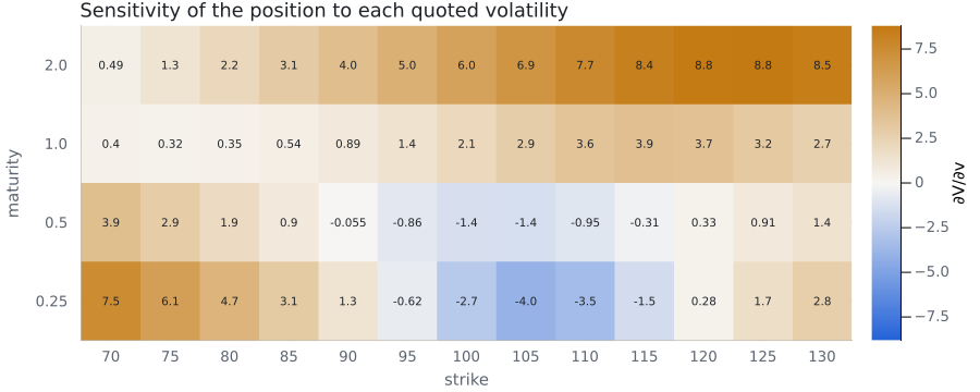

The chain rule, written out, gives the same numbers: the sensitivities of the price to the parameters, at the calibrated point, times those of the parameters to the quotes.

p = calibrated(vols)
∂p_∂v = ForwardDiff.jacobian(calibrated, vols)
maximum(abs, vec(∂V_∂v) - transpose(∂p_∂v) * ForwardDiff.gradient(price, p))

4.884981308350689e-15

The test suite also checks the gradient of an Asian option against recalibrating and repricing with a quote moved both ways.

Caveats

• The derivative is that of the Monte Carlo estimator, with its own statistical error: more paths make it converge to the derivative of the price, and the same seed for the two sides of a finite difference makes the check above meaningful.
• The pathwise derivative misses what moves a discontinuity of the payoff: the knock-out of a barrier, the jump of a binary option. Their sensitivities from the pathwise derivative are biased; the likelihood ratio and Vibrato estimators of VibratoMonteCarlo.jl are the remedy for the payoffs they cover.
• The calibrated Heston of this example does not satisfy the Feller condition ($2 \kappa \theta < \sigma^2$), so the simulated variance reaches its floor, and the price has kinks in the parameters. The derivative is exact between them, but a finite difference that crosses them is not: a check needs small bumps ($10^{-6}$ in volatility).