Calibration

The problem

The market quotes prices $m_1, \dots, m_n$ of European options with strikes $K_i$ and maturities $T_i$: here 13 strikes on each of four maturities, out of the money (puts below the forward, calls above it), whose prices hold no intrinsic value. Their implied volatilities $v_i$ invert the formula of Black and Scholes $C_{bs}$: $C_{bs}(S_0, K_i, r, T_i, v_i, d) = m_i$.

A model with parameters $p$ gives the prices $C_i(p)$, computed with pricer: one smile per maturity, all of its strikes from one set of evaluations of the characteristic function, and the maturities by broadcasting. Their implied volatilities $\sigma_i(p)$ are the model volatilities, and the calibration minimises the volatility errors

\[e_i(p) = \sigma_i(p) - v_i, \qquad L(p, v) = \frac{1}{2} \sum_{i=1}^n e_i(p)^2 .\]

Volatilities rather than prices put the errors of all the strikes on one scale: the price of a far out of the money option is a small number, and an error on it of the size of the error at the money would be a large error in volatility.

The model is Heston's, with the variance $V$ of the log-price mean-reverting at the speed $\kappa$ to the level $\theta$,

\[\frac{dS_t}{S_t} = (r - d)\,dt + \sqrt{V_t}\,dW_t, \qquad dV_t = \kappa (\theta - V_t)\,dt + \sigma \sqrt{V_t}\,dZ_t, \qquad d\langle W, Z\rangle_t = \rho\,dt, \qquad V_0 = \sigma_0^2,\]

and parameters $p = (\sigma, \sigma_0, \kappa, \rho, \theta)$, in the order of HestonProcess(σ, σ₀, λ, κ, ρ, θ, underlying) with no market price of volatility risk ($\lambda = 0$). Its characteristic function has a closed form (Heston, 1993), in the formulation of Albrecher et al., continuous in the maturity, see References. The quotes are generated by the model itself, with $p = (0.5, 0.2, 1.5, -0.7, 0.04)$, and their prices are moved by up to 1%, which no Heston model fits exactly.

using FinancialFFT, FinancialMonteCarlo, FinancialToolbox, ForwardDiff, LinearAlgebra

S0, r, d = 100.0, 0.02, 0.01
zero_rate = ZeroRate(r)
maturities = [0.25, 0.5, 1.0, 2.0]
strikes = collect(70.0:5.0:130.0)
forward(T) = S0 * exp((r - d) * T)
# out of the money: puts below the forward, calls above
smiles = [FinancialMonteCarlo.EuropeanOptionSmile(T, strikes, strikes .>= forward(T)) for T in maturities]
quote_T = repeat(maturities; inner = length(strikes))
quote_K = repeat(strikes, length(maturities))
quote_call = quote_K .>= forward.(quote_T)

method = CosMethod(2^9)
heston(p) = HestonProcess(p[1], p[2], zero(p[1]), p[3], p[4], p[5], Underlying(S0, d))
model_prices(p) = reduce(vcat, pricer.(heston(p), zero_rate, method, smiles))
implied_vols(prices) = blsimpv.(S0, quote_K, r, quote_T, prices, d, quote_call)

p_market = [0.5, 0.2, 1.5, -0.7, 0.04]
market_prices = model_prices(p_market) .* (1 .+ 0.01 .* sin.(1:length(quote_K)))
v = implied_vols(market_prices)

The parameters are constrained: $\sigma$, $\sigma_0$, $\kappa$ and $\theta$ are positive, and $|\rho| < 1$. The search runs on unconstrained variables $x$, with $p = (e^{x_1}, e^{x_2}, e^{x_3}, \tanh x_4, e^{x_5})$, so that every step gives a valid model.

Derivatives of the model volatilities

The model volatility $\sigma_i(p)$ solves $C_{bs}(S_0, K_i, r, T_i, \sigma_i, d) = C_i(p)$. By the implicit function theorem its derivatives are those of the price, divided by the vega $\nu_i = \partial_\sigma C_{bs}$ at $\sigma_i$:

\[\frac{\partial \sigma_i}{\partial p_j} = \frac{1}{\nu_i} \frac{\partial C_i}{\partial p_j},\]

and this is how the rules of blsimpv differentiate it, without going through the iterations of its solver. The Jacobian $J = \partial_x e$ of the errors, an $n \times 5$ matrix, is then one evaluation of the pricer in dual numbers with five partials: ForwardDiff carries them through the characteristic exponent, the cosine series of CosMethod (its truncation range is a constant) and the implied volatility. Forward mode suits a Jacobian with fewer columns than rows; reverse mode (Zygote, Mooncake) gives the gradient $J^\top e$ of the loss in one backward pass, which suits a quasi-Newton method on the loss instead.

Levenberg–Marquardt

Gauss–Newton linearises the errors around the current point, $e(x + \delta) \approx e(x) + J \delta$, and takes the least squares solution of $J \delta = -e$, i.e. the solution of the normal equations $J^\top J \delta = -J^\top e$. It converges fast near a solution with small errors, but far from it the linear model can be wrong, and a step can increase the loss. Levenberg and Marquardt add a damping $\mu > 0$:

\[\left(J^\top J + \mu D\right) \delta = -J^\top e, \qquad D = \operatorname{diag}\left(J^\top J\right).\]

For $\mu \to 0$ the step is the Gauss–Newton one; for a large $\mu$ it is a short step along the gradient $-J^\top e$ of the loss, scaled by $D$ (Marquardt's choice, which makes the step independent of the units of the parameters), and decreases the loss. $\mu$ is adapted: divided after a step that decreases the loss, which is accepted, and multiplied after one that does not, which is rejected. From a starting point far from the quotes the method converges in fewer than 20 iterations, each a Jacobian and a pricing.

to_p(x) = [exp(x[1]), exp(x[2]), exp(x[3]), tanh(x[4]), exp(x[5])]
to_x(p) = [log(p[1]), log(p[2]), log(p[3]), atanh(p[4]), log(p[5])]
vol_errors(x, v) = implied_vols(model_prices(to_p(x))) .- v
function calibrate(v; x = to_x([0.3, 0.25, 1.0, -0.3, 0.06]), μ = 1e-2, iterations = 100)
    e = vol_errors(x, v)
    for _ in 1:iterations
        J = ForwardDiff.jacobian(t -> vol_errors(t, v), x)
        A = Array(transpose(J) * J)   # the 5 × 5 system on the CPU, also when J is on the GPU
        δ = -(A + μ * Diagonal(diag(A))) \ Array(transpose(J) * e)
        e_new = vol_errors(x + δ, v)
        if sum(abs2, e_new) < sum(abs2, e)
            x, e, μ = x + δ, e_new, μ / 3   # accepted: closer to Gauss-Newton
            norm(δ) < 1e-12 && break        # converged
        else
            μ *= 4                          # rejected: closer to gradient descent
            μ > 1e12 && break               # no step decreases the loss: at the rounding floor
        end
    end
    return x
end
x = calibrate(v)
p = to_p(x)
(market = p_market, calibrated = p, rms_error = sqrt(sum(abs2, vol_errors(x, v)) / length(v)))

(market = [0.5, 0.2, 1.5, -0.7, 0.04], calibrated = [0.4974756436373531, 0.20032202363123203, 1.499721321133487, -0.70150772699676, 0.0399190110357729], rms_error = 0.0006294941839189739)

The root mean square error is about 6 basis points of volatility, from prices moved by up to 1%:

model_vols = implied_vols(model_prices(p))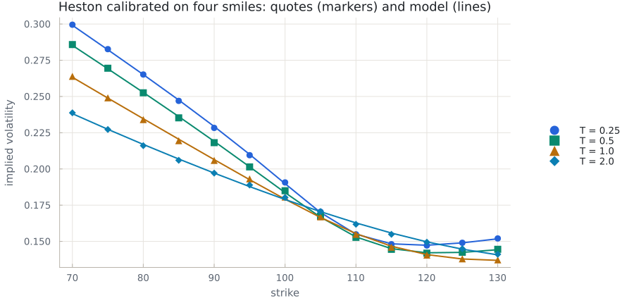

Identifiability

How well the quotes determine the parameters shows in the singular values of $J$: near the optimum the loss is about $\frac{1}{2} \|e + J \delta\|^2$, so a move $\delta$ along a right singular vector of $J$ changes the volatilities by its singular value times $\|\delta\|$. A small singular value is a combination of parameters that the quotes hardly see.

J = ForwardDiff.jacobian(t -> vol_errors(t, v), x)
F = svd(J)
(singular_values = F.S, weakest_direction = F.V[:, end])

(singular_values = [0.833227168966429, 0.3351443909700158, 0.22227337991501697, 0.12761525433170867, 0.03823462789985819], weakest_direction = [-0.24812655982714876, -0.02768820957426461, -0.9568185237500169, 0.0028773315816633554, 0.14885095542428678])

The weakest direction, in the variables $x = (\log \sigma, \log \sigma_0, \log \kappa, \operatorname{artanh} \rho, \log \theta)$, is mostly $\log \kappa$, with the volatility of the variance and the level $\theta$ compensating it: the speed of mean reversion shows only in how the smile changes with the maturity, and four maturities up to two years see it weakly. A calibration to fewer maturities, or to noisier quotes, leaves $\kappa$ undetermined; fixing it, or adding a penalty on it to the loss, are the usual remedies.

Sensitivity of the calibrated parameters to the quotes

How do the calibrated parameters $x^*$ move when a quoted price moves? The implicit function theorem gives the derivatives of the calibration without differentiating the solver. At the optimum the gradient of the loss vanishes,

\[g(x^*, v) = \partial_x L(x^*, v) = J^\top e(x^*) = 0,\]

and where $\partial_x g$ is invertible

\[\frac{\partial x^*}{\partial v} = -\left(\partial_x g\right)^{-1} \partial_v g = H^{-1} J^\top, \qquad H = \partial^2_x L = J^\top J + \sum_{i=1}^n e_i \, \partial^2_x e_i ,\]

since $\partial_v g = -J^\top$. $H$ is the Hessian of the loss, from ForwardDiff with nested dual numbers, through the pricer and the implied volatility. The quoted volatilities depend on the prices through the inverse of the vega, $\partial v_i / \partial m_i = 1 / \nu_i$ and $\partial v_i / \partial m_j = 0$ for $i \neq j$, and the parameters on $x$ through the diagonal Jacobian of the change of variables, so that

\[\frac{\partial p^*}{\partial m} = \frac{\partial p}{\partial x} \, H^{-1} J^\top \operatorname{diag}\left(\frac{1}{\nu_1}, \dots, \frac{1}{\nu_n}\right),\]

a $5 \times n$ matrix from derivatives at the optimum only.

H = ForwardDiff.hessian(t -> sum(abs2, vol_errors(t, v)) / 2, x)
vegas = blsvega.(S0, quote_K, r, quote_T, v, d)
∂x_∂m = (H \ transpose(J)) ./ transpose(vegas)
∂p_∂x = ForwardDiff.jacobian(to_p, x)
∂p_∂m = ∂p_∂x * ∂x_∂m
size(∂p_∂m)

(5, 52)

A check on one quote, the put with strike 85 at one year, against moving its price by a cent both ways, implying the volatilities again and recalibrating, and against the Gauss–Newton approximation $H \approx J^\top J$, which drops the term of the errors:

i, h = 30, 1e-2
up, down = copy(market_prices), copy(market_prices)
up[i] += h
down[i] -= h
recalibrated = (to_p(calibrate(implied_vols(up); x = x)) - to_p(calibrate(implied_vols(down); x = x))) / 2h
gauss_newton = ∂p_∂x * (((transpose(J) * J) \ transpose(J)) ./ transpose(vegas))
(implicit = ∂p_∂m[:, i], recalibrated = recalibrated, gauss_newton = gauss_newton[:, i])

(implicit = [-0.014969078567403737, -0.00016140216730970445, -0.20746041383999106, -0.0063584204042946265, 0.0015223454602898432], recalibrated = [-0.014969104101589248, -0.00016140389712121506, -0.20746083819748184, -0.006358426855379573, 0.0015223470720089616], gauss_newton = [-0.014898859791464854, -0.0001614428027877028, -0.20687681267318792, -0.006337026446068048, 0.001521014790520503])

The implicit derivatives match the recalibration to about five digits, the accuracy of the finite difference: a recalibration stops at the rounding floor of the volatilities (about $10^{-13}$), where the loss no longer decreases measurably, and along the weakest direction, where the loss is flattest, that leaves its solution uncertain to about $10^{-8}$; a smaller move of the price would magnify that, a larger one the curvature. The implicit derivatives have neither error, and cost one Hessian instead of two calibrations per quote. When the model fits the quotes exactly the errors vanish, $H = J^\top J$ and the sensitivities are the pseudo-inverse of $J$; with the 1% noise of these quotes the second term moves them by about half a percent.

On the GPU

With CUDA.jl loaded, the same code runs on the GPU once the method and the quotes are there: each smile is priced on the device (see GPU), the implied volatilities are a broadcast of blsimpv over CuArrays, and ForwardDiff differentiates both, so the Jacobian is a CuArray too. Only the $5 imes 5$ system of each step comes back to the CPU, which is what the Array in calibrate is for:

using CUDA
method = CosMethod(2^9; mode = FinancialMonteCarlo.CudaMode())
quote_T, quote_K, quote_call = CuArray(quote_T), CuArray(quote_K), CuArray(quote_call)
market_prices = model_prices(p_market) .* (1 .+ 0.01 .* sin.(CuArray(1:length(quote_K))))
x = calibrate(implied_vols(market_prices))