Methods

Every method is a configurator struct passed to pricer, in the place of the MonteCarloConfiguration of FinancialMonteCarlo.jl. All of them price every payoff and model of the package.

All of them agree with the closed formula of Black and Scholes:

using FinancialFFT, FinancialMonteCarlo, FinancialToolbox

S0, K, r, d, T, σ = 100.0, 105.0, 0.02, 0.01, 1.1, 0.2
model = BlackScholesProcess(σ, Underlying(S0, d))
zero_rate = ZeroRate(r)
option = EuropeanOption(T, K)
exact = blsprice(S0, K, r, T, σ, d)

methods = [LewisMethod(600.0, 20000), CosMethod(2^12), CarrMadanLewisMethod(600.0, 16), CarrMadanMethod(400.0, 18), CosDensityMethod(), FFTDensityInverter()]
[nameof(typeof(method)) => abs(pricer(model, zero_rate, method, option) - exact) for method in methods]

6-element Vector{Pair{Symbol, Float64}}:
          :LewisMethod => 4.440892098500626e-15
            :CosMethod => 2.7533531010703882e-14
 :CarrMadanLewisMethod => 1.5504317829595493e-9
      :CarrMadanMethod => 6.586247991435812e-9
     :CosDensityMethod => 5.763203247965976e-10
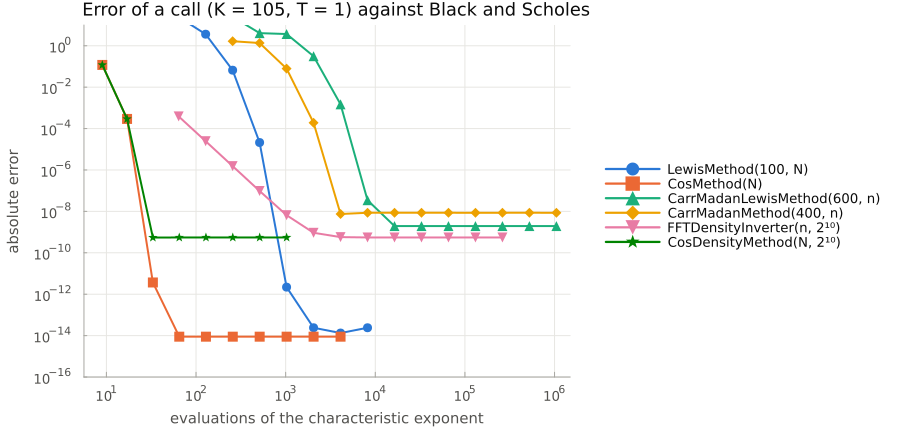
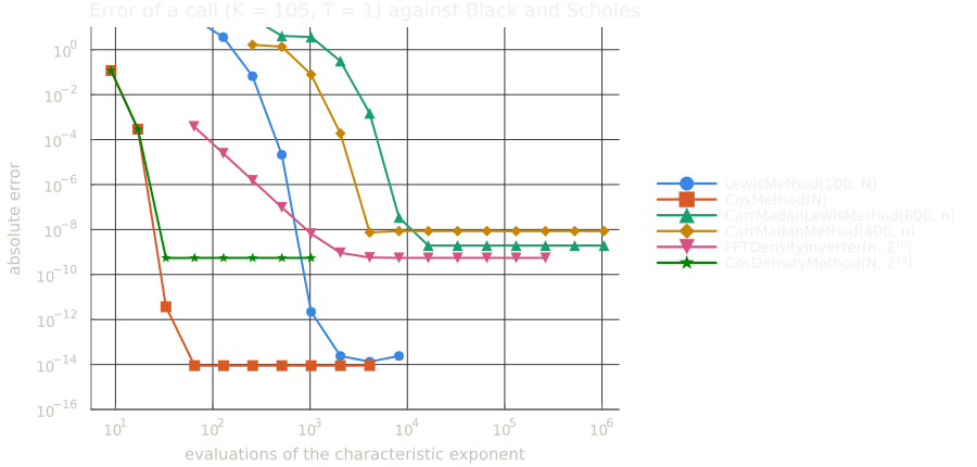
   :FFTDensityInverter => 5.764340116343192e-10

The error depends on how many times a method evaluates the characteristic exponent, which is most of its cost. COS converges exponentially and reaches the rounding floor with a few dozen terms; Lewis does too, once its nodes cover the decay of the integrand; the Carr-Madan methods stop at the error of the interpolation on the strike grid, and the two density methods at the error of Simpson's rule on M intervals:

Choosing a method

• LewisMethod and CosMethod are the most accurate, and with CosDensityMethod and FFTDensityInverter the only ones whose Zygote gradients can be relied upon, see Automatic differentiation.
• CosMethod has no range parameter: its range comes from the tails of the model and covers the forward of every strike. A smile shares one range, so all of its strikes reuse the same coefficients, at the price of a larger N when the strikes are many standard deviations apart. It expands the put and recovers the call by parity, so calls stay accurate on models with a heavy right tail. On the CPU the strikes of a smile share the phases of the characteristic function, and each strike sums the series with a Clenshaw recurrence, at the cost of one sincos instead of one cos per term: in Black Scholes with N = 2^12, a smile of 100 strikes costs about 3.5 times a single option, rather than about 18. On the GPU the series stays one broadcast over terms and strikes.
• LewisMethod evaluates the characteristic function on the nodes in [0, A] only, since the integrand is even. It prices the strikes of a smile from one set of these evaluations: on the CPU each strike sums the quadrature with a Clenshaw recurrence (in Reinsch's form, which stays accurate at the money), at the cost of one sincos per strike instead of an exp and a cos per node, about 6 times faster for smiles of 100-500 strikes with N = 20000.
• CarrMadanLewisMethod and CarrMadanMethod run one FFT for all strikes, so their cost does not grow with the number of strikes; prices between the nodes of the strike grid come from Lagrange polynomials on six nodes, of order h⁶ in the step h = 2π / A of the grid, which is what limits their accuracy. The interpolant is continuous but its derivatives in the strike jump at the nodes, by about 1e-8 for CarrMadanLewisMethod(600, 16).
• CarrMadanMethod needs A / 2^Npow to be small with respect to the damping, which is capped by the exponential moments of the model.
• CosDensityMethod and FFTDensityInverter price with their density, the cosine expansion and the FFT inversion: they need no range parameter, and the strikes of a smile share the density, so a smile costs one density and one Simpson's rule per strike. Their error is the one of Simpson's rule on M intervals (about 1e-9 with the default M = 2^10), and they are slower than CosMethod, which integrates the payoff exactly against the cosine expansion: their purpose is to price with the densities that other estimators use.

model = MertonProcess(σ, 5.0, 0.03, 0.02, Underlying(S0, d))
pricer(model, zero_rate, FFTDensityInverter(), option) - pricer(model, zero_rate, LewisMethod(600.0, 20000), option)

5.515481404927414e-10

Floating-point types

Prices have the floating-point type of the model, the rates and the payoff: the grids, the truncation ranges and the parameters of the method (A, α, given in Float64 in the examples) are converted to it, so Float32 inputs give Float32 prices and BigFloat inputs BigFloat prices. FFTW transforms Float32 and Float64 only: in other types the FFT methods use a radix-2 FFT of the package, slower but in their precision. The truncation range of the COS methods comes from a tail probability of 1e-14 in Float64, scaled by the machine epsilon in other types: in BigFloat the range is wider, so reaching its precision needs a larger N (and M for CosDensityMethod).

setprecision(BigFloat, 128) do
    model = BlackScholesProcess(BigFloat(0.2), Underlying(BigFloat(100), BigFloat(0.01)))
    pricer(model, ZeroRate(BigFloat(0.02)), CosMethod(2^10), EuropeanOption(BigFloat(1), BigFloat(100)))
end

Densities

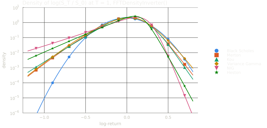
density returns the density of the log-return log(S_T / S_0), for estimators that need it without a closed formula, such as the likelihood ratio method or Vibrato. Like pricer, it dispatches on the method:

The setup runs once, then the density is evaluated at any number of points: f(y) at a point, on the CPU, and FinancialFFT.density_values(f, y) at an array of points, on the GPU too. It does not depend on S_0, so the density of log(S_T) given S_t is f(x - log(S_t)); outside its range [f.a, f.b] it is zero.

f = density(model, zero_rate, FFTDensityInverter(), T)
f(0.1), f.a, f.b

(1.5412478817694935, -1.7806255733811118, 1.9095445780880056)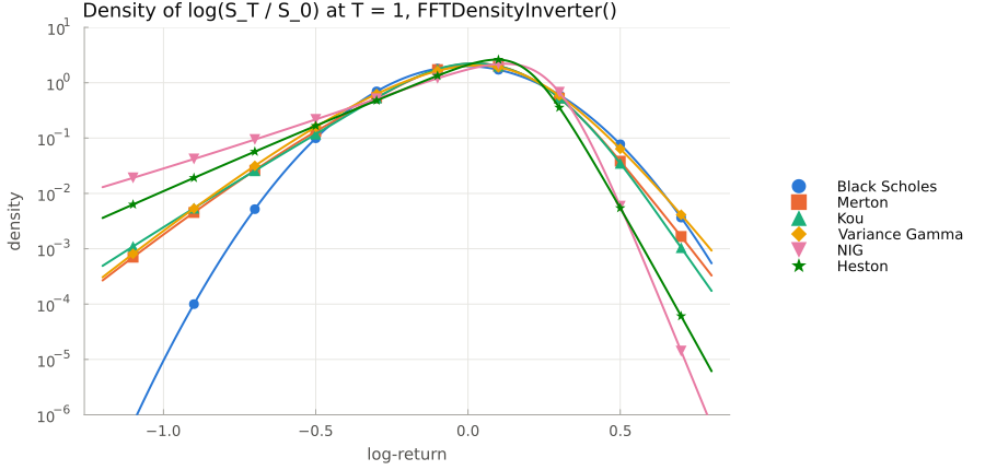

The density is generic in the number type of the model, so its scores, the weights of the likelihood ratio method, come from automatic differentiation of log(f(y)); the range is a constant for differentiation:

using ForwardDiff

merton(s) = MertonProcess(s, 5.0, 0.03, 0.02, Underlying(S0, d))
score(y) = ForwardDiff.derivative(s -> log(density(merton(s), zero_rate, FFTDensityInverter(), T)(y)), σ)
score(0.1)

-3.591227230504311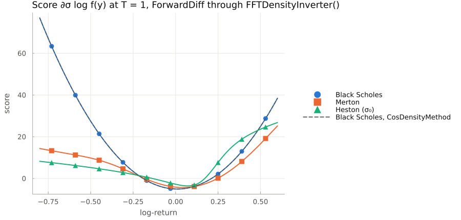

• FFTDensityInverter is the one to use for many evaluations, e.g. one per path of a simulation: its interpolation is a gather of four values. Its error is of order dx⁴ (about 1e-13 with the default N = 14 in Black and Scholes), and the grid narrows with the horizon, so short steps keep their resolution. Every AD back-end differentiates it, Zygote included, on the CPU and on the GPU.
• CosDensityMethod converges exponentially on smooth densities, and is the most accurate of the three there; it struggles where the density is not smooth, as Variance Gamma over a short step, whose density has a cusp at its mode (2% off with 512 terms, against 6e-6 for FFTDensityInverter(16)).

All errors are absolute: far in the tails, where the density is close to the floor of the machine epsilon, the relative error, which is the one of a score, grows.