FinancialFFT.jl

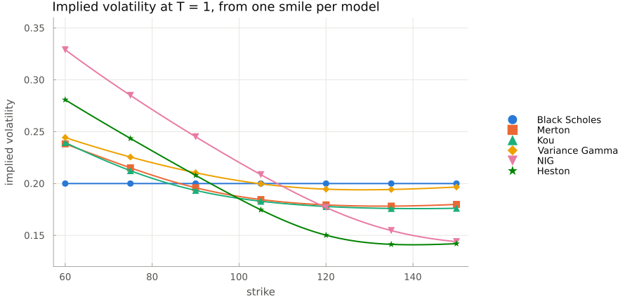
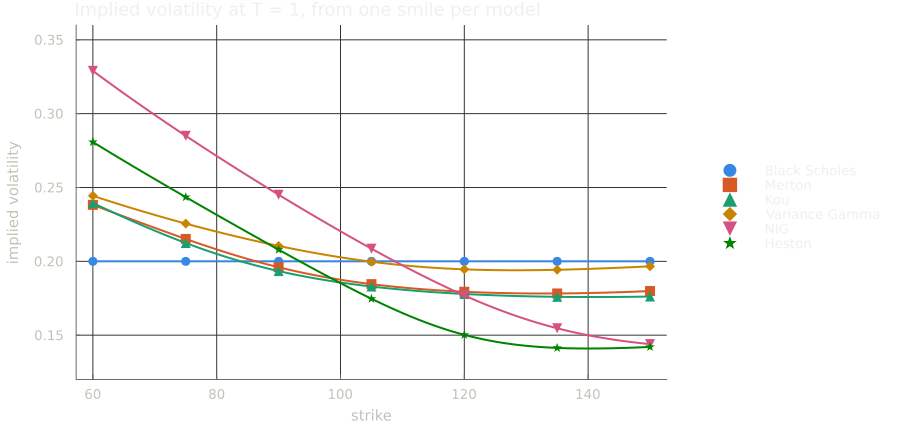
FinancialFFT.jl prices European options from the characteristic function of the log-price. A model enters only through its characteristic exponent, so pricing Merton, Kou, Variance Gamma, NIG or Heston costs about as much as Black and Scholes: a quadrature, a cosine series or an FFT, with no simulation noise. Prices are generic in the number type, so every Greek comes from automatic differentiation, and the same code runs on the GPU.

Implied volatility smiles of six models

Relation to FinancialMonteCarlo.jl

The package adds methods to the pricer of FinancialMonteCarlo.jl, and uses its types for everything else: the model (BlackScholesProcess, HestonProcess, …), the underlying (Underlying), the curve (ZeroRate) and the payoff (EuropeanOption, BinaryEuropeanOption, and their smiles). The last-but-one argument picks the numerical method, so moving a European option from simulation to a Fourier method changes one argument:

pricer(model, zero_rate, MonteCarloConfiguration(10^6, 1), option)  # Monte Carlo, FinancialMonteCarlo.jl
pricer(model, zero_rate, CosMethod(2^12), option)                    # COS method, FinancialFFT.jl

Features

Pricing methods: LewisMethod, CosMethod, CarrMadanLewisMethod, CarrMadanMethod, CosDensityMethod and FFTDensityInverter, compared in Methods.
Densities of the log-return through density, for the likelihood ratio method and Vibrato: CosDensityMethod and FFTDensityInverter, see Densities.
Models: Black–Scholes, Merton, Kou, Variance Gamma, Normal Inverse Gaussian, Heston.
Payoffs: European and binary (digital) options, calls and puts, and their smiles (several strikes, one maturity), with every method. Options with different maturities are priced by broadcasting, pricer.(model, zero_rate, method, options).
Non-constant zero rates and dividends.
Automatic differentiation with DualNumbers.jl, HyperDualNumbers.jl, ForwardDiff.jl, ReverseDiff.jl, Zygote.jl, Mooncake.jl and TaylorSeries.jl, see Automatic differentiation for the exceptions.
Float32 and BigFloat prices, see Floating-point types.
GPU execution through CUDA.jl, see GPU.

Installation

] add FinancialFFT

Quick start

using FinancialFFT, FinancialMonteCarlo

S0, K, r, d, T, σ = 100.0, 100.0, 0.02, 0.01, 1.0, 0.2

model = BlackScholesProcess(σ, Underlying(S0, d))
zero_rate = ZeroRate(r)
option = EuropeanOption(T, K)

pricer(model, zero_rate, LewisMethod(600.0, 20000), option)

8.349405767096759

The same call works with any other method and model:

model = MertonProcess(σ, 5.0, 0.03, 0.02, Underlying(S0, d))
pricer(model, zero_rate, CosMethod(2^12), option)

8.969890962447508

GPU

With CUDA.jl loaded, passing FinancialMonteCarlo.CudaMode() as the last argument of pricer evaluates the characteristic function and the integrals on the GPU:

using CUDA
smile = FinancialMonteCarlo.EuropeanOptionSmile(T, CuArray([90.0, 100.0, 110.0]), CuArray([true, true, false]))
pricer(model, zero_rate, CosMethod(2^12), smile, FinancialMonteCarlo.CudaMode())

Every method runs on the GPU, with the accuracy it has on the CPU.
density(model, zero_rate, method, T, FinancialMonteCarlo.CudaMode()) computes the density on the GPU with FFTDensityInverter and CosDensityMethod, and FinancialFFT.density_values evaluates it there at a CuArray of points, differentiable with ForwardDiff.jl and Zygote.jl.
The strikes of a smile must be on the device. A single option is given as on the CPU.
ForwardDiff.jl and Zygote.jl differentiate the prices on the GPU. ReverseDiff.jl and Mooncake.jl are not supported on the GPU.

Testing

] test FinancialFFT

The GPU tests are not part of the default run; on a machine with a CUDA GPU they run with the following command, which adds CUDA.jl to the test environment:

using Pkg
Pkg.test("FinancialFFT"; test_args = ["gpu"])