Methods

Vibrato prices American options too, when the payoff is an AmericanOption or a BinaryAmericanOption, see American options. The two conditional methods are not exported: they are the exact inner integration limit of Vibrato and VibratoSaltando on the same paths, mostly test oracles, and only price European and binary options.

All of them agree with the closed formula of Black and Scholes, here for a binary call and its delta:

using VibratoMonteCarlo, FinancialMonteCarlo, FinancialToolbox, HyperDualNumbers

S0 = hyper(100.0, 1.0, 1.0, 0.0)
K, r, d, T, σ = 105.0, 0.02, 0.01, 1.0, 0.2
model = BlackScholesProcess(σ, Underlying(S0, d))
zero_rate = ZeroRate(r)
option = BinaryEuropeanOption(T, K)
mc = MonteCarloConfiguration(50_000, 10; sampling = FinancialMonteCarlo.AntitheticMC())
exact = blsbin(S0, K, r, T, σ, d)

methods = [Vibrato(mc, VibratoMonteCarloGaussLegendre()), PureLRM(mc, VibratoMonteCarloGaussLegendre()), VibratoMonteCarlo.Conditional(mc)]
errors(price) = (value = price.value - exact.value, delta = price.epsilon1 - exact.epsilon1, gamma = price.epsilon12 - exact.epsilon12)
[nameof(typeof(method)) => errors(pricer(model, zero_rate, method, option)) for method in methods]

3-element Vector{Pair{Symbol, @NamedTuple{value::Float64, delta::Float64, gamma::Float64}}}:
     :Vibrato => (value = -0.0006129958408715996, delta = 5.459145404413182e-5, gamma = 2.1383913577990637e-5)
     :PureLRM => (value = 2.3314683517128287e-15, delta = 1.734723475976807e-17, gamma = -6.749158523722265e-18)
 :Conditional => (value = -0.0006129958408721548, delta = 5.459145404413182e-5, gamma = 2.138391357799214e-5)

PureLRM on Black and Scholes is one integral against the density at maturity: with Gauss-Legendre it is exact up to rounding, and the Monte Carlo configuration only provides the seed.

Inner integrations

The inner expectation of every method but the conditional ones is an integral of the payoff against a density, on the standardized variable of the last step. The integration is the second argument of the method:

The payoff has a kink (a call) or a jump (a binary) at the strike. Split at the strike, every piece of the Gauss-Legendre rule has a smooth integrand and converges exponentially; across the jump, Gauss-Hermite, a uniform grid and Monte Carlo converge slowly:

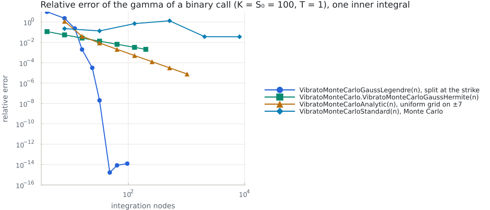
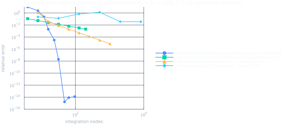
Gauss-Legendre is therefore the default choice on Gaussian laws. The FFT density of the Lévy processes, through Vibrato, PureLRM and American options, and of Heston through PureLRM, needs VibratoMonteCarloAnalytic: it comes from FFTDensityInverter of FinancialFFT.jl, evaluated by FinancialFFT.density_values at all the nodes of a path in one call. Its trapezoid is not split at the strike, so a binary payoff converges only linearly in the node spacing (2-3% on the value of a binary with the 200 default nodes on Kou and Heston, ten times less with 2000), and derivatives that live in the tails of the density, as the one over the vol of vol of Heston, need wider bounds than ±7 standard deviations (±10 for 1e-6).

Choosing a method

• On Black and Scholes and Heston, Vibrato with VibratoMonteCarloGaussLegendre. On Black and Scholes PureLRM is exact and needs no simulation.
• On Kou and Merton, VibratoSaltando: the last step is exact and at least one time step long. It does not differentiate over the jump intensity $\lambda$ or the maturity $T$: it warns.
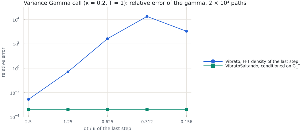
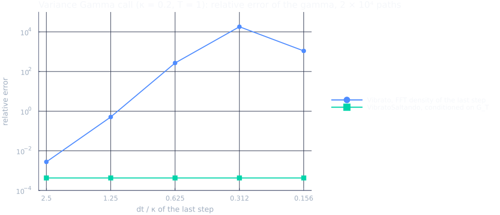
• On Variance Gamma and Normal Inverse Gaussian, VibratoSaltando: conditioned on the subordinator, it is exact for any Nstep, and it differentiates over $\kappa$ and $T$ too. The FFT Vibrato needs a smooth density of the last step, which the Variance Gamma density is only for $dt / \kappa \gtrsim 2.5$:

On Kou and Merton, VibratoSaltando with SobolMC or AntitheticMC applies them to the jumps as well: each path takes a fixed number of uniforms, the number of jumps and their sizes by inversion of their laws, the times as sorted uniforms (a path with more jumps than the cap, at probability $10^{-9}$, draws them from the generator). Sobol uses the coordinates after those of the diffusion, antithetic pairs the reflected uniforms. FinancialMonteCarlo's own paths of Kou and Merton still draw their jumps from the generator (FinancialMonteCarlo.jl#34). On Variance Gamma and Normal Inverse Gaussian both apply to $G_T$, drawn by inversion.

Smiles

A smile of strikes with one maturity is priced on the same paths, with one price per strike:

smile = FinancialMonteCarlo.EuropeanOptionSmile(T, [90.0, 100.0, 110.0], [false, true, true])
prices = pricer(model, zero_rate, Vibrato(mc, VibratoMonteCarloGaussLegendre()), smile)
[(value = p.value, delta = p.epsilon1, gamma = p.epsilon12) for p in prices]

3-element Vector{@NamedTuple{value::Float64, delta::Float64, gamma::Float64}}:
 (value = 3.2648414053387835, delta = -0.24618378184092157, gamma = 0.015684766790981988)
 (value = 8.34665673466196, delta = 0.5538910139645941, gamma = 0.01965686377548631)
 (value = 4.5668230562653145, delta = 0.3676316186729985, gamma = 0.018677936072249626)

American options

Vibrato prices an option exercisable at the Nstep dates of the time grid, with the exercise policy of Longstaff-Schwartz. On Black and Scholes the policy is fixed in price space and every exercise date is integrated with the likelihood ratio method over a Brownian bridge, so that the gamma is unbiased for the policy:

put = AmericanOption(T, K, false)
price = pricer(model, zero_rate, Vibrato(MonteCarloConfiguration(20_000, 10), VibratoMonteCarloGaussLegendre()), put)
(value = price.value, delta = price.epsilon1, gamma = price.epsilon12)

(value = 10.233872183830146, delta = -0.5422863334056294, gamma = 0.020194285179964327)

On Lévy processes and Heston the exercise decisions are frozen when differentiating: value and delta are accurate, the gamma misses the term of the exercise boundary and is biased low, see American options.

Limits

These are limits of the methods, measured against the Lewis formula, not defects:

• With VibratoMonteCarloStandard the gammas are noisier than with quadrature: up to about 4% at $10^5$ paths and Nstep = 300, where values and deltas are within 2e-3.
• The bounds of VibratoMonteCarloAnalytic must reach far enough in the upper tail, where a call payoff is large: at ±5 standard deviations the volga of a Variance Gamma call was 3-45% off, at ±7 (the default) it is within noise.
• VibratoSaltando on Variance Gamma, with $a = T / \kappa$: the $n$-th $S_0$ derivative of a call at $K = S_0 e^{(r - d - \psi) T}$ exists only for $a > (n - 1) / 2$, and the estimator has finite variance only for $a > n - 1$. This is the smoothness of the true price, not of the estimator.
• Derivatives over $\kappa$ through the law of $G_T$ are the noisiest: at $5 \cdot 10^5$ paths the standard deviation of $\partial_\kappa$ is 3% on Variance Gamma and 1.2% on NIG.
• Vibrato on American options on Black and Scholes has an unbiased gamma, but its variance grows with Nstep.